
Estimating Typhoon Uwan’s Exposure – A Manual Analysis Under Pressure #
Characteristics of the exercise #
Type of trainings exercise:
This exercise can be used in online and presence training.
It can be done as a follow-along exercise or individually as a self-study.
It works well as a scenario exercise: participants play the GIS team of a National Society in the first days of a typhoon emergency.
Exercise Track:
This exercise is part of the Philippines Typhoon Response Exercise Track
Estimated time demand for the exercise
Tasks 1–6 (hazard zone): approx. 30 minutes
Tasks 7–13 (population and health sites): approx. 60 minutes
Tasks 14–16 (visualisation, prior impact, export): approx. 45 minutes
Discussion: 20–30 minutes
Aim of the exercise: In this exercise you will estimate, step by step and without a model, how many people and how many health facilities lie within 200 km of the track of Typhoon Uwan (Fung-wong, November 2025). Finally, you will flag which provinces had already been hit by Typhoon Tino a few days earlier, because these are the places where response capacity is most stretched.
Instructions for the trainers #
Trainers Corner
Prepare the training
Take the time to familiarise yourself with the exercise and the provided material. Run through all tasks once yourself and note down your results. They will be useful as reference values for participants (see Results).
Prepare a white-board. It can be either a physical whiteboard, a flip-chart, or a digital whiteboard (e.g. Miro board) where the participants can add their findings and questions.
Before starting the exercise, make sure everybody has installed QGIS and has downloaded and unzipped the data folder.
Ask participants about their computer specifications beforehand. The population raster for the whole Philippines is a few hundred MB. On slow machines, consider providing a raster already cut to Luzon.
Check out How to do trainings? for some general tips on facilitating trainings.
Conduct the training
Introduction (scenario briefing):
Introduce the context (see the Context box below). Make clear that participants are standing at the beginning of the emergency: the earthquake and Typhoon Tino have already happened, and Typhoon Uwan is approaching.
Before opening QGIS, ask the group:
Which operations have you been part of where information management helped you, or where it was missing?
What can we do with GIS at this stage of the emergency?
What would the different sectors or clusters (shelter, health, food security and livelihoods, logistics) need to know from us?
Which data would we need, and where could we find it? Collect the answers on the whiteboard and compare them afterwards with the datasets in the folder.
Do we have a 3W (Who does What Where) map? Where would we look for previous situation reports?
Short comment: if a map is only available as an image or PDF (for example in a situation report), the Georeferencer can be used to bring it into QGIS.
Follow-along:
Show and explain each step yourself at least twice and slow enough so everybody can see what you are doing, and follow along in their own QGIS-project.
Make sure that everybody is following along and doing the steps themselves by periodically asking if anybody needs help or if everybody is still following.
Be open and patient to every question or problem that might come up. Your participants are essentially multitasking by paying attention to your instructions and orienting themselves in their own QGIS-project.
Many participants will create a buffer for the first time in Task 6. Take a moment to explain what a buffer is before moving on. When you get to the note after Task 6, point out that the 200 km buffer is a simplification and show where to find the literature on wind radii.
Tasks 8 to 12 repeat the same logic for different datasets. Once participants have understood the population steps, faster participants can continue on their own while you support the others.
Wrap up:
Use the discussion questions in the Results section.
Point out that every step done manually here can later be automated with the Model Designer (see the Madagascar exercise track).
Leave some time for open questions.
Trainers Corner: Preparing the data folder
The data folder should follow the standard folder structure. The following files are expected in data/input (paths relative to this folder). The file names below are the names used in the instructions; rename the downloaded files accordingly.
File name in exercise |
How to prepare it |
|---|---|
|
Download the last3years lines shapefile ( |
|
Download the shapefile version of the administrative boundaries from HDX (COD-AB Philippines) and unzip it. We use admin level 2 (provinces, |
|
Download the constrained population count raster at 100 m resolution from HDX (WorldPop Philippines). |
|
Export health facilities for the Philippines with the HOT Export Tool (or download them from healthsites.io). Keep the fields |
optional: |
For the optional vulnerability extension: WorldPop age and sex structures. Use the 1 km version to save space. |
Note: 2025 storms are still provisional tracks in IBTrACS and are usually replaced by reanalysed best tracks within about two years. If you rebuild the data folder later, check whether the track or the wind radii fields (used in the optional wind radii method) have changed.
Available Data #
Download all datasets here, save the folder on your computer and unzip the file.
The folder contains the whole standard folder structure with all data in the input folder and the additional documentation in the documentation folder.
Note
All intermediate results of this exercise are saved in the data → interim folder. In some versions of the folder structure, this folder is called temp. If you have a temp folder instead, use that one.
Dataset |
Source |
Description |
|---|---|---|
Tropical cyclone tracks |
International Best Track Archive for Climate Stewardship (IBTrACS) |
The tracks of all storms worldwide of the last three years as lines. Each line segment contains the storm name, time, wind speed and the wind radii reported by the different agencies. Tracks from 2025 are provisional. |
Administrative boundaries |
Province boundaries (admin level 2) of the Philippines, provided by OCHA. |
|
Population |
Estimated number of people per 100 m grid cell for 2015 (constrained to built-up areas). This is a modelled dataset, not a census count. |
|
Health facilities |
Health facilities from OpenStreetMap. Completeness depends on how well an area has been mapped. |
Context

It is 7 November 2025. About a month ago, a magnitude 6.9 earthquake struck Cebu. Between 4 and 5 November, Typhoon Tino (Kalmaegi) made multiple landfalls across the Visayas and Palawan, causing flooding, landslides and widespread damage. Volunteers, staff and relief stocks are already committed to these two operations.
Now a second storm, Typhoon Uwan (Fung-wong), is intensifying east of the Philippines and heading towards Luzon. The Philippine Red Cross has just activated its Early Action Protocol for typhoons. Interestingly, the protocol was not activated for Tino a week earlier.
You work in the information management team of the Philippine Red Cross. The operations team asks you one question:
Where will Uwan hit people and health services the hardest, and which of these places are already struggling after Tino?
There is no time to build an automated model. You have to do the analysis by hand, quickly and in a way you can explain to the operations team.
Reports on the events
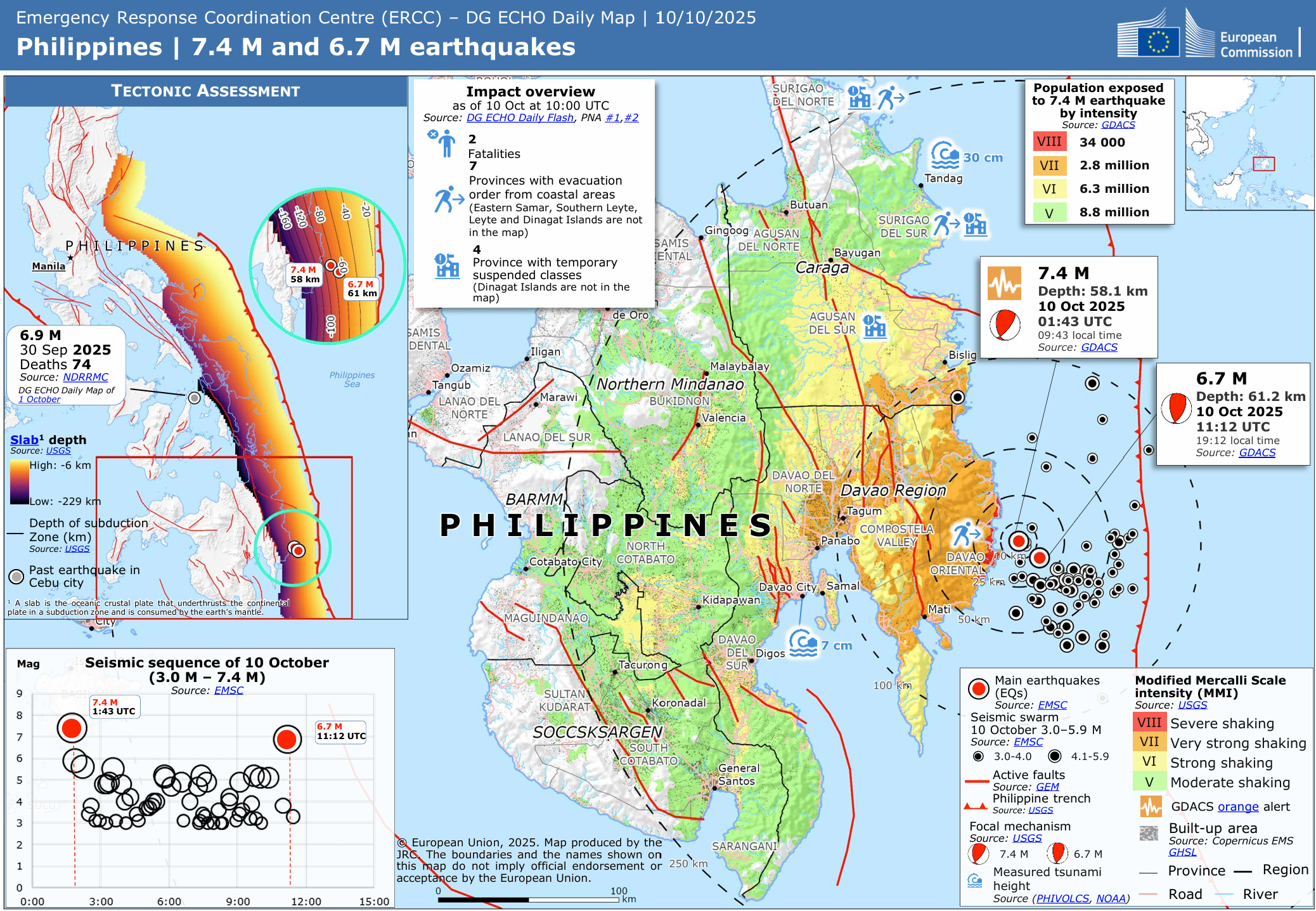
ERCC – DG ECHO Daily Map of the 7.4 M and 6.7 M earthquakes off Mindanao, 10 October 2025. The inset also shows the 6.9 M Cebu earthquake of 30 September. Source: European Commission, JRC.#
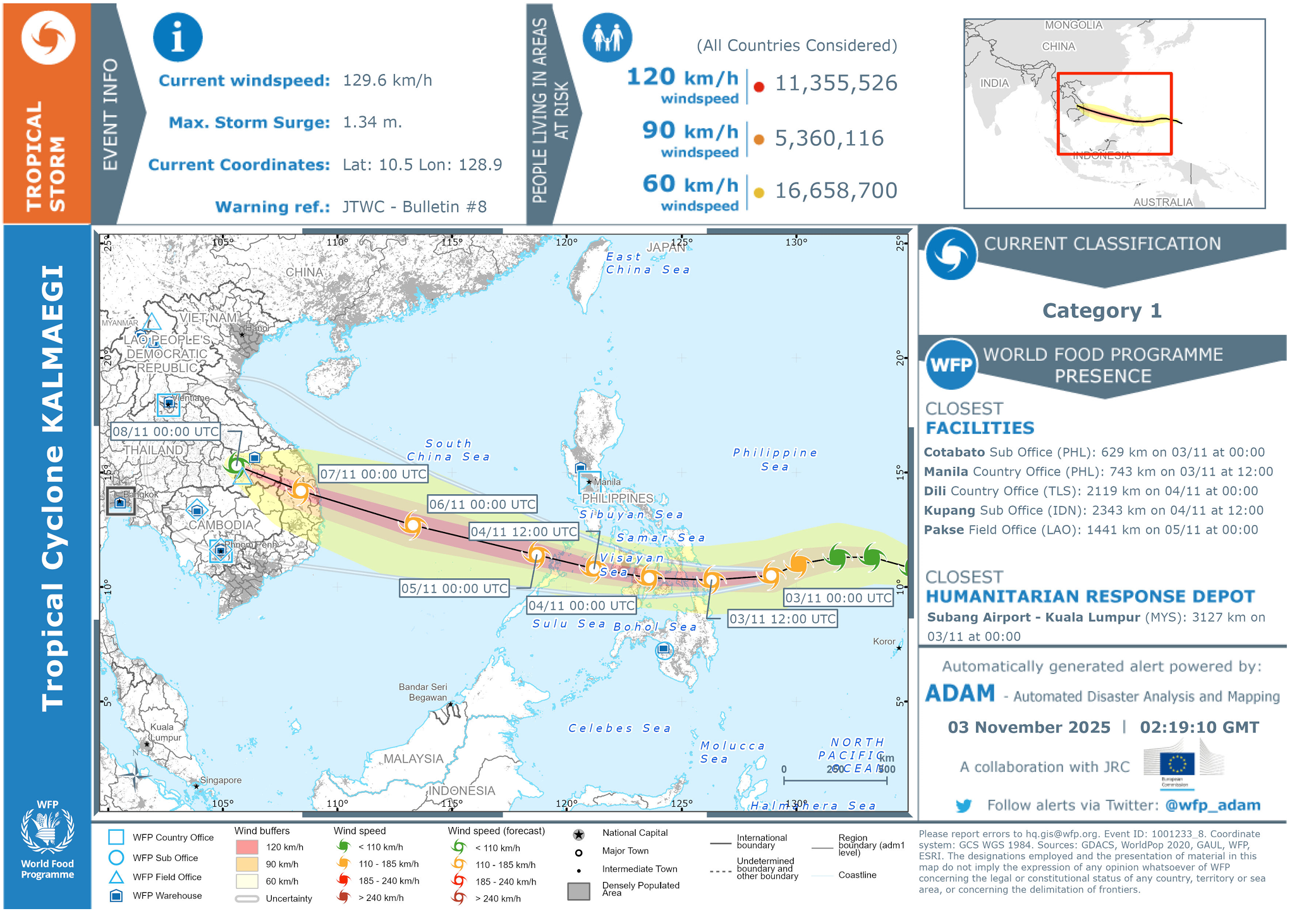
ADAM alert for Tropical Cyclone Kalmaegi (Tino), 3 November 2025, with wind buffers of 60, 90 and 120 km/h. Source: WFP ADAM, in collaboration with JRC.#
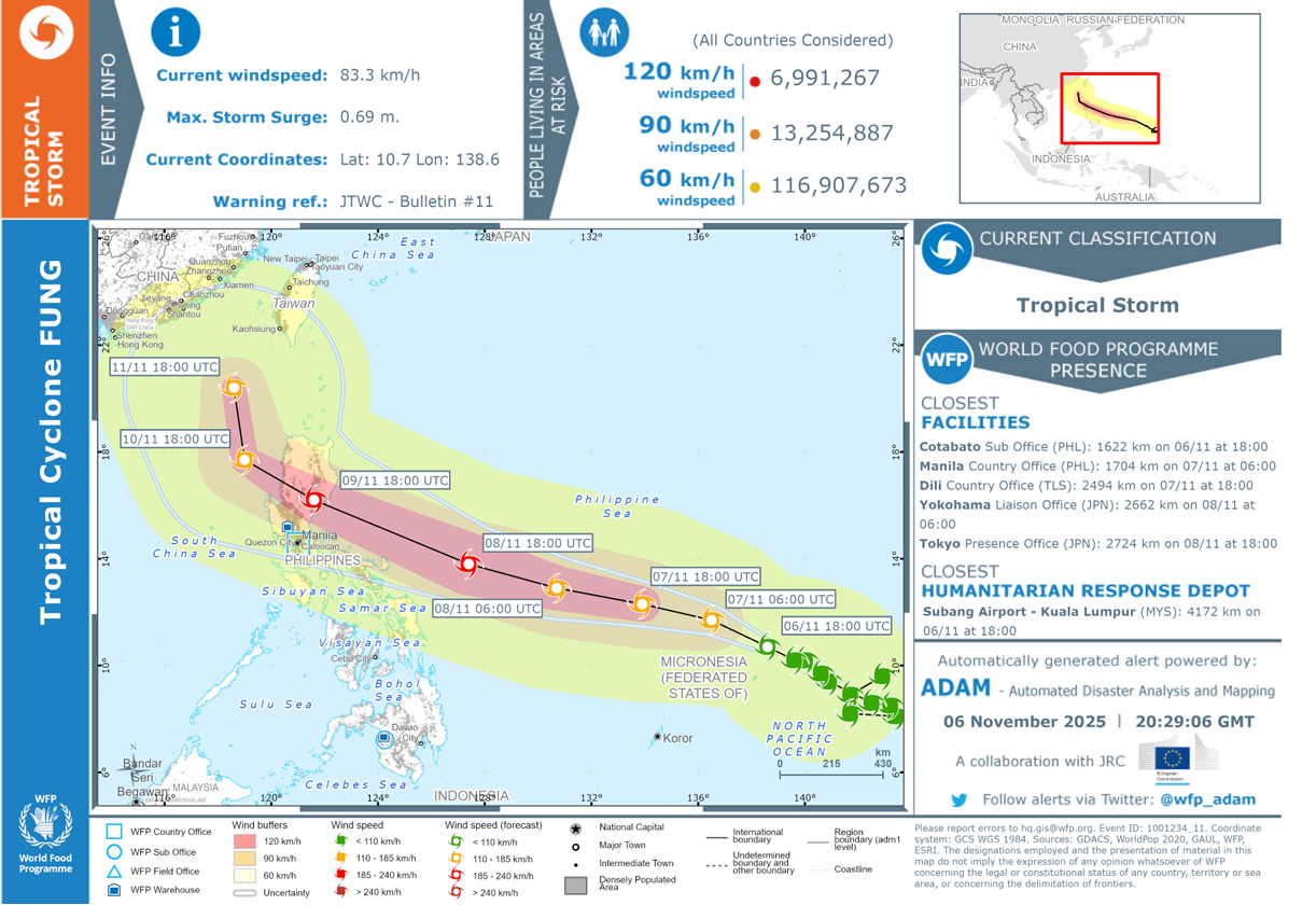
ADAM alert for Tropical Cyclone Fung-wong (Uwan), 6 November 2025, with wind buffers of 60, 90 and 120 km/h. Source: WFP ADAM, in collaboration with JRC.#
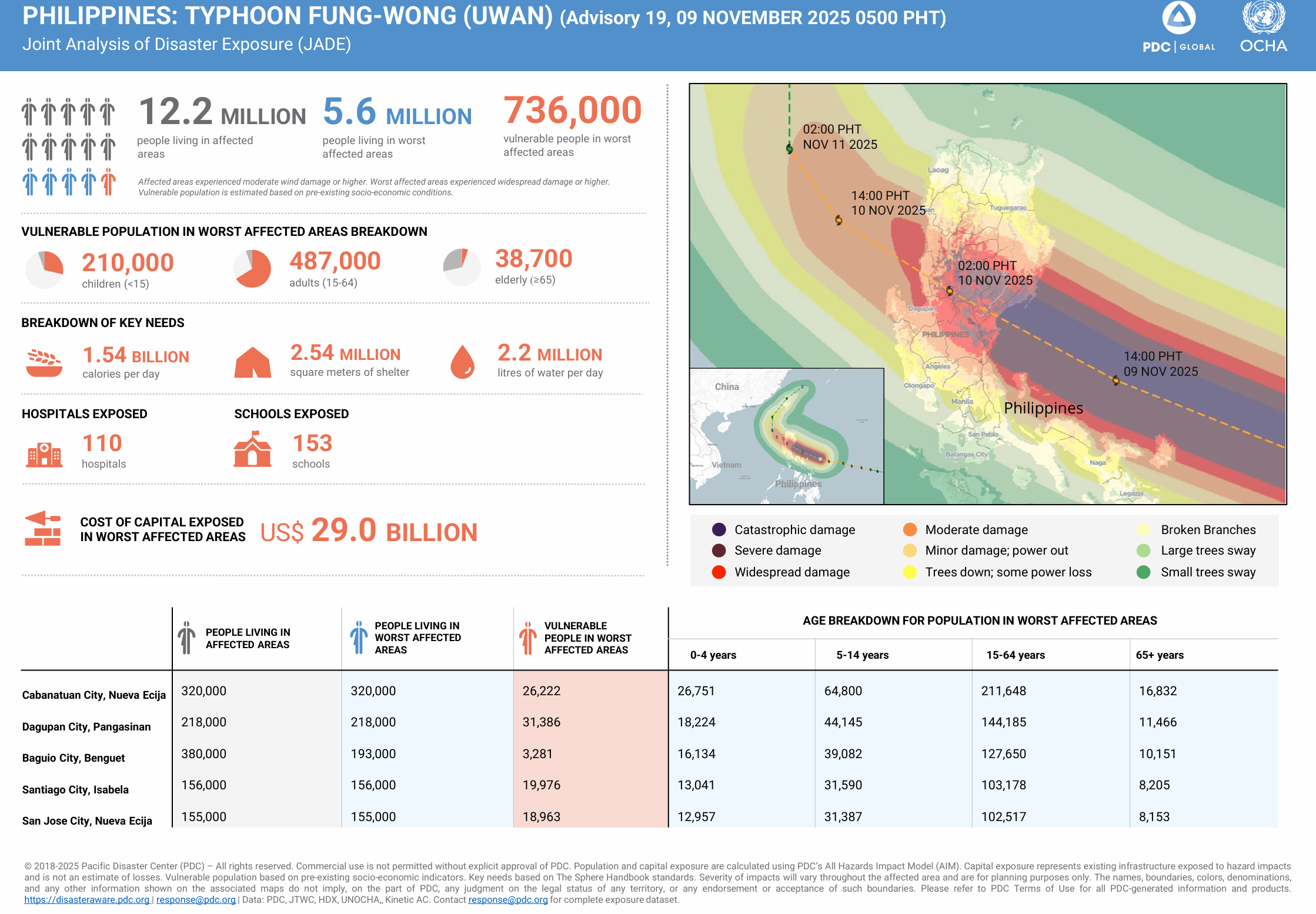
Joint Analysis of Disaster Exposure (JADE) for Typhoon Fung-wong (Uwan), advisory 19, 9 November 2025. Source: PDC Global and OCHA.#
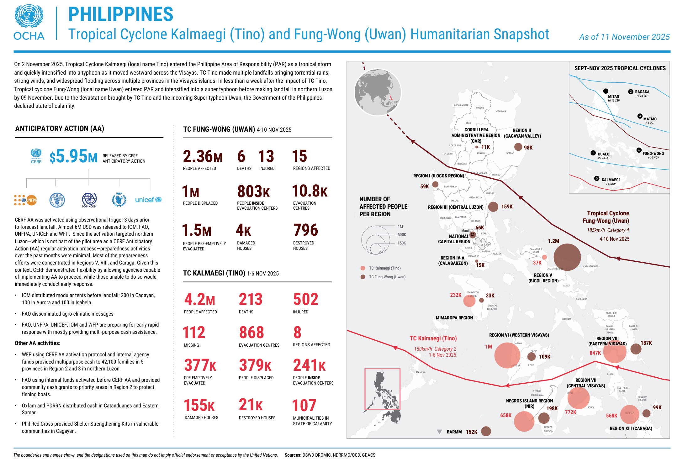
Humanitarian snapshot of Tropical Cyclones Kalmaegi (Tino) and Fung-wong (Uwan), as of 11 November 2025. Source: OCHA.#
Note
In this exercise we use the observed IBTrACS track of Uwan and treat it as if it were the latest forecast. In a real operation you would work with forecast tracks and wind fields from PAGASA, JTWC or JMA, which change with every update.
Tasks: #
Part A – Preparing the hazard: from storm track to hazard zone#
Open QGIS and create a new project by clicking on
Project→New.Save the project in the
projectfolder. Click onProject→Save as, navigate to the folder and name the projectTyphoon_Uwan_Exposure.Add the OpenStreetMap basemap for orientation. Click on
Layer→Add Layer→Add XYZ Layer..., selectOpenStreetMapand clickAdd. Alternatively, openXYZ Tilesin theBrowserpanel and double-click onOpenStreetMap(Wiki basemap). Keep the basemap at the bottom of the Layers panel.Load the storm tracks and find Uwan:
Load
IBTrACS.last3years.list.v04r01.lines.shpfromdata→input→IBTrACS.last3years.list.v04r01.linesby drag and drop (Wiki Video).Open the attribute table and look at the fields. Find
NAME,ISO_TIME(time in UTC) andUSA_WIND(maximum wind speed in knots).The layer contains every storm worldwide of the last three years. Untick the box next to
IBTrACS.last3years.list.v04r01.linesin the Layers panel to make it invisible while we filter it.Right-click on
IBTrACS.last3years.list.v04r01.lines→Filter.... The Query Builder opens.In the
Fieldslist, double-click onNAME. It appears in the expression box at the bottom.Click on the
=button.Under
Values, click onAll. This loads all storm names in the dataset.Type
FUNGin the search field underValuesand double-click onFUNG-WONG. The expression now reads"NAME" = 'FUNG-WONG'.Click
OK.Tick the box next to
IBTrACS.last3years.list.v04r01.linesagain. Only the track of Uwan is now visible. The filter icon next to the layer name shows that the layer is filtered. Processing tools only use the features that pass the filter, so every tool we run on this layer from now on only works with Uwan.Save the filtered track as its own file. Like this, we do not change the
IBTrACS.last3years.list.v04r01.lineslayer, and we can always come back to it and filter it again.Right-click on
IBTrACS.last3years.list.v04r01.lines→Export→Save Features As…Format:
GeoPackageFile name: click on the
…button, navigate todata→interimand name the fileStorm_Track_Fung_Wong.Layer name: change it to
Storm_Track_Fung_Wong.Make sure
Add saved file to mapis ticked and clickOK.
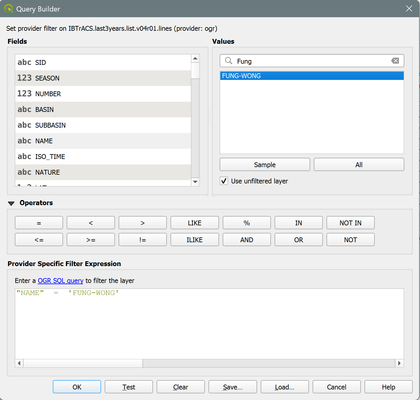
The query builder in QGIS 3.44 to filter the storm tracks.#
Tip
Uwan is the local Philippine name (assigned by PAGASA). IBTrACS uses the international name, Fung-wong. Storm names are reused over the years, so when you work with the full IBTrACS archive, always combine the name with the season, e.g. "SEASON" = 2025 AND "NAME" = 'FUNG-WONG'. If the filter returns nothing, check the spelling of the name in the attribute table.
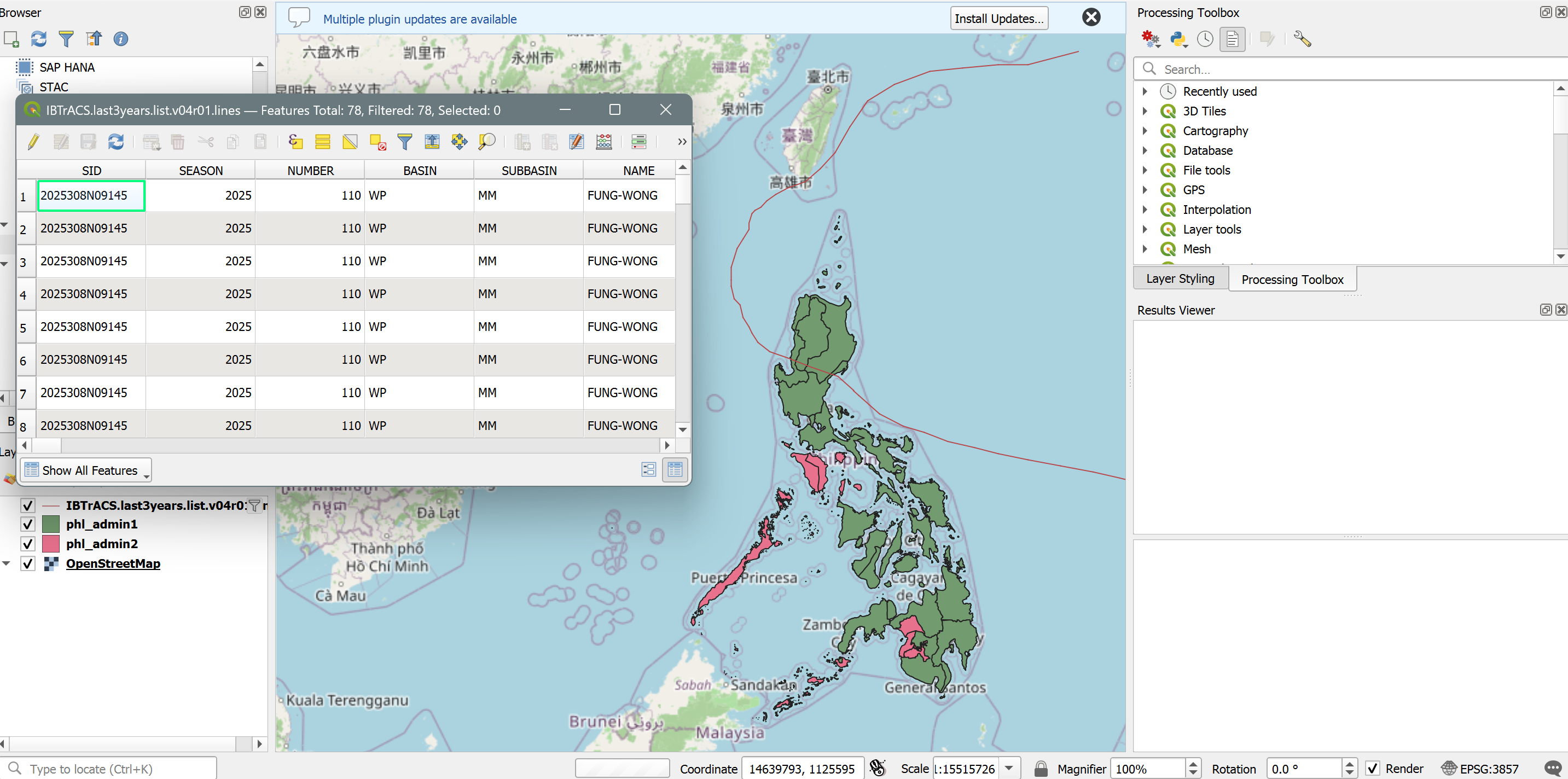
Your QGIS map canvas should resemble this.#
Reproject the storm track to a CRS that uses metres. The IBTrACS data is in degrees, and a buffer distance in kilometres can only be calculated correctly in a CRS that measures in metres.
In the Processing Toolbox, search for
Reproject Layer.Input:
Storm_Track_Fung_WongTarget CRS:
EPSG:32651(WGS 84 / UTM zone 51N, which covers Luzon)Save the result in the
interimfolder asStorm_Track_Fung_Wong_32651
Attention
Buffer distances must be calculated in a CRS that measures in metres. The IBTrACS data uses EPSG:4326, which measures in degrees. Always reproject to a projected CRS before buffering.
Buffer the storm track. A buffer is a zone of a fixed distance around a feature. Here we draw a zone of 200 km around the track and treat everything inside it as exposed to the storm.
In the Processing Toolbox, search for
Buffer.Input:
Storm_Track_Fung_Wong_32651Distance:
200and set the unit next to it tokilometersSegments: leave default (5)
Dissolve result:
YesSave the output in the
interimfolder asUwan_Buffer_200km
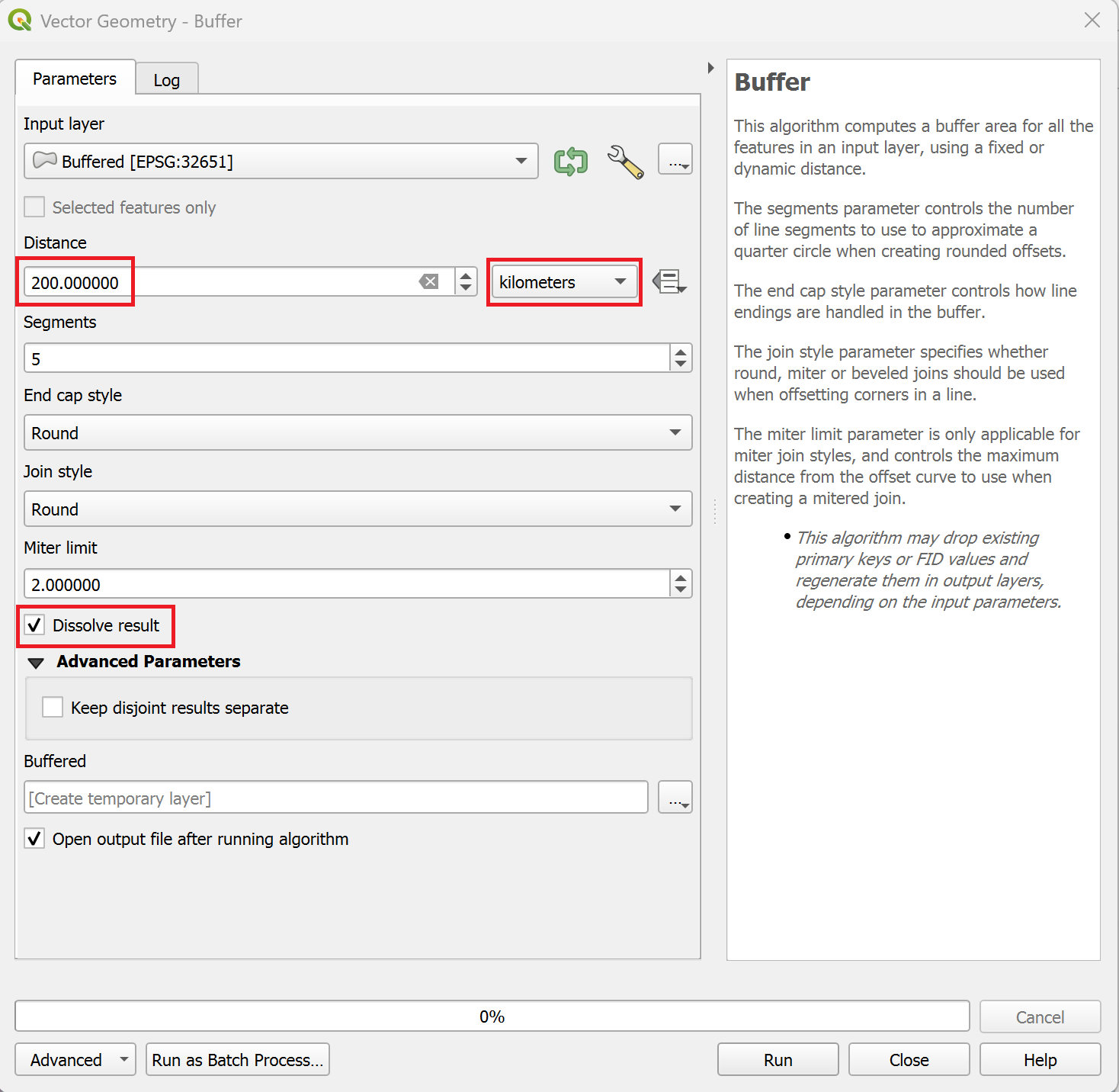
Buffer dialogue for the storm track in QGIS 3.44.#
Intermediate Result: Buffer
The intermediate result shows the track of Uwan and a 200 km wide zone on each side of it. The buffer must be a single feature.
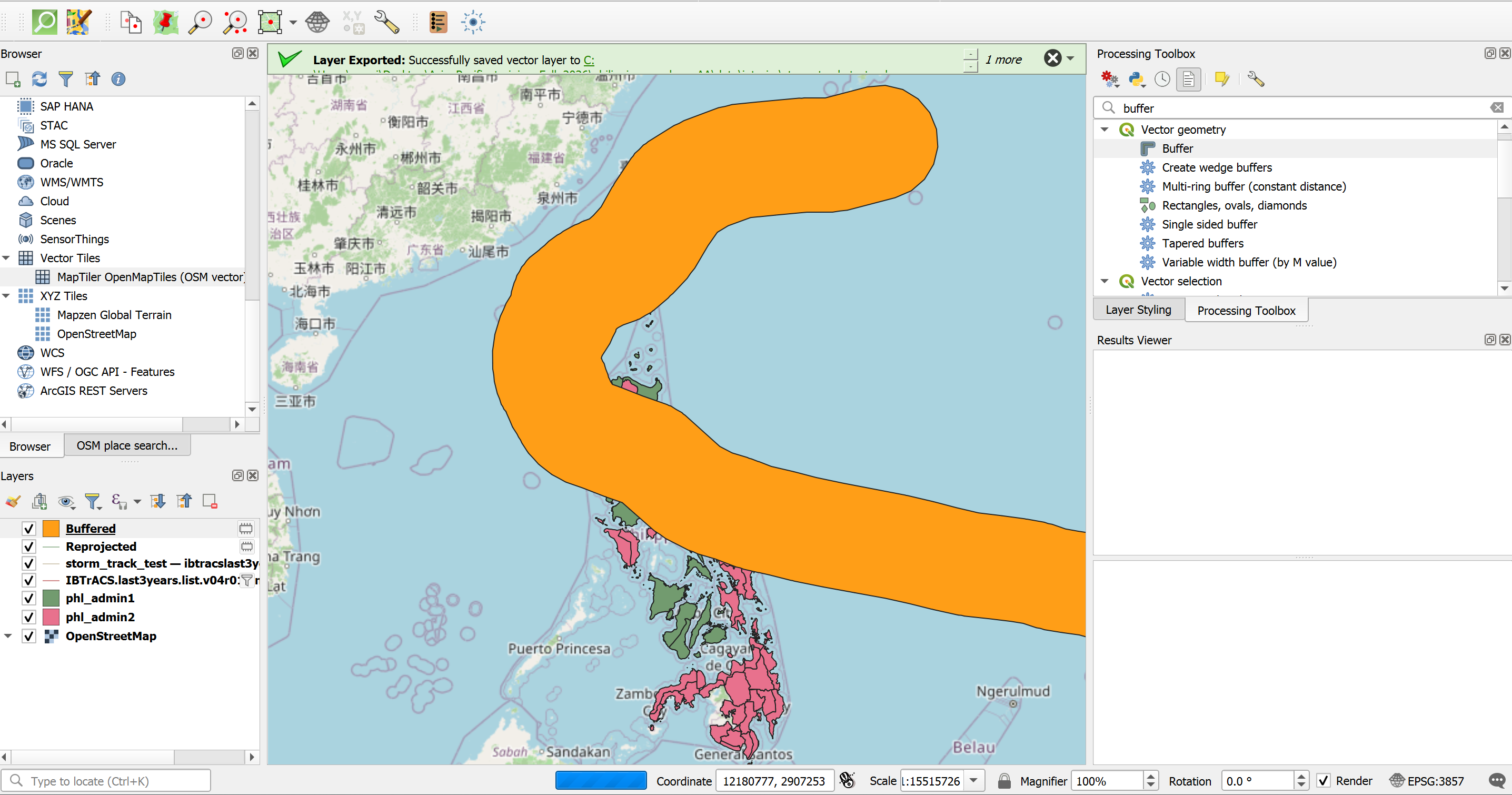
Your buffer should look similar to the picture.#
Note: The 200 km buffer is a simplification
A real wind field is not the same width along the whole track. It grows and shrinks as the storm develops, and it is not symmetric: in the northern hemisphere, the strongest winds are usually on the right side of the track. Forecasting agencies therefore report wind radii, which give the distance from the storm centre to which winds of a certain speed (e.g. 34, 50 and 64 knots) reach in each of four quadrants. Operational products, such as GDACS or the ADAM alerts of the World Food Programme, use modelled wind fields to show zones of different wind speeds.
For this exercise we keep it quick and use one fixed buffer, so that you first understand what a buffer does. If you want to learn more about wind radii, have a look at:
IBTrACS v04r01 column documentation (NOAA NCEI): definitions of the wind radii fields
USA_R34_*,USA_R50_*andUSA_R64_*.Tropical Cyclones effects (GDACS): how GDACS estimates the wind impact of tropical cyclones from the forecast bulletins.
Holland, G. J. (1980): An analytic model of the wind and pressure profiles in hurricanes. Monthly Weather Review, 108, 1212–1218. The classic model of the wind profile of a tropical cyclone, used by many wind field models.
Knaff, J. A. et al. (2007): Statistical tropical cyclone wind radii prediction using climatology and persistence. Weather and Forecasting, 22, 781–791. How wind radii are forecast and how much they vary between storms.
Going further: Wind zones from the reported wind radii (optional)
Instead of one fixed 200 km buffer, you can use the size of the wind field that was reported along the track. IBTrACS gives the 34-knot radius (gale-force winds, about 63 km/h) and the 64-knot radius (typhoon-force winds, about 118 km/h) for four quadrants (NE, SE, SW, NW), in nautical miles. Each line segment of the track carries the wind radii reported at its start.
Calculate the wind radii in metres.
Open the Field Calculator on the layer
Storm_Track_Fung_Wong_32651.Create a new field: name
r34_m, typeDecimal number (real).Expression:
max(
  coalesce("USA_R34_NE", 0),
  coalesce("USA_R34_SE", 0),
  coalesce("USA_R34_SW", 0),
  coalesce("USA_R34_NW", 0)
) * 1852
Click
OK.Repeat the same for a field
r64_m, replacingR34withR64in all four field names.Save your edits and switch off editing mode.
Buffer the track with the wind radii (34-knot zone):
In the Processing Toolbox, search for
Buffer.Input:
Storm_Track_Fung_Wong_32651Distance: click the Data defined override button next to the distance field, choose
Field type: int, doubleand selectr34_m.Segments: leave default (5)
Dissolve result:
YesSave the output in the
interimfolder asUwan_Zone_34kt
Repeat the buffer for the 64-knot zone using the field
r64_m. Save the output asUwan_Zone_64kt.
The 34-knot zone is a corridor along the track that changes its width as the storm develops. The 64-knot zone is a much narrower corridor in its centre and only exists where Uwan had typhoon strength. You can run Part B with these two zones instead of Uwan_Buffer_200km and compare the results.
Why max, coalesce and 1852?
1852converts nautical miles to metres (1 nautical mile = 1852 m).max(...)takes the largest of the four quadrants. This turns the asymmetric wind field into a circle that is as large as the widest quadrant. It is a cautious simplification, because the real wind field is not a circle.coalesce(field, 0)replaces missing values with 0. Early and late parts of a storm often have no wind radii, and withoutcoalescethe whole result would become empty (NULL).
Part B – Who and what is exposed?#
Great, you now have the area that is potentially exposed to Typhoon Uwan! But the operations team does not plan with buffers. They need to know how many people are potentially exposed and where they are. In this part we therefore combine the buffer with the administrative boundaries and find out, for every province, how much of the population lies inside the buffer and which health facilities, especially hospitals, are potentially exposed to the coming typhoon.
We add the results one after another to the province layer. Each processing step creates a new layer that contains all previous columns plus the new one, so at the end you have one layer with all results.
Load the base data:
phl_admin2.shpfromdata→input→admin_boundaries→phl_admin_boundaries.shpphl_pop_2015_CN_100m_R2025A_v1.tiffromdata→input→worldpop(Layer→Add Layer→Add Raster Layer)
Calculate the total population per province. We need it later to calculate what share of each province’s population is exposed.
In the Processing Toolbox, search for
Zonal Statistics.Input layer:
phl_admin2Raster layer:
phl_pop_2015_CN_100m_R2025A_v1Field prefix:
pop_total_Statistics to calculate:
SumonlySave the output in the
interimfolder asadmin2_pop_sum
Clip the population raster to the buffer:
In the Processing Toolbox, search for
Clip Raster by Mask Layer.Input layer:
phl_pop_2015_CN_100m_R2025A_v1Mask layer:
Uwan_Buffer_200kmSave the output in the
interimfolder asUwan_Pop_200km
Tip
The population raster is in EPSG:4326 and the buffer is in EPSG:32651. Clip Raster by Mask Layer handles the difference automatically. If you run into problems, reproject the buffer to EPSG:4326 first, as done in the Madagascar exercise.
Intermediate Result: Clipped population
Only the population inside the 200 km buffer should remain visible.
Calculate the exposed population per province:
Run
Zonal Statisticsagain.Input layer:
admin2_pop_sumRaster layer:
Uwan_Pop_200kmField prefix:
pop200_Statistics:
SumSave as
admin2_pop_exposed
Calculate the share of exposed people. Open the Field Calculator on
admin2_pop_exposedand create a new decimal fieldpop200_pct:round("pop200_sum" / "pop_total_sum" * 100, 1)
Provinces that are completely outside the buffer have no value (
NULL) inpop200_sum, so they also getNULLinpop200_pct. Read these as 0 % exposed.
Why look at both numbers?
The absolute number (pop200_sum) shows where most people are affected, which matters for the size of the response. The percentage (pop200_pct) shows which provinces are hit almost completely, which matters because neighbouring areas in the same province cannot easily support them. A large province with many exposed people and a small province where nearly everyone is exposed can both be priorities, for different reasons.
Count the exposed health facilities.
Load
phl_healthsites_osm.gpkg.In the Processing Toolbox, search for
Extract by location.Extract features from:
phl_healthsites_osmWhere the features:
intersectBy comparing to the features from:
Uwan_Buffer_200kmSave as
Uwan_Healthsites_200kmIn the Processing Toolbox, search for
Count points in polygon.Polygons:
admin2_pop_exposed, Points:Uwan_Healthsites_200km, Count field name:hs200. Save the result in theoutputfolder asUwan_Exposure_Provinces.
Look at the hospitals in the buffer. Open the attribute table of
Uwan_Healthsites_200km. UseSelect by expressionwith"amenity" = 'hospital'to see which hospitals lie within the buffer. Hospitals close to the track are the facilities whose functioning is most at risk and which the health team should contact first.
Note
OpenStreetMap coverage in the Philippines is comparatively good because of many past mapping activities, but it is not complete. A province with zero health facilities in the result may simply be poorly mapped. Compare with official facility lists (e.g. from the Department of Health) where possible.
Part C – Making the results usable#
Visualise the exposed population.
Right-click on
Uwan_Exposure_Provinces→Properties→Symbology.Change
Single SymboltoGraduated.Value:
pop200_sumColour ramp: e.g.
RedsMode: e.g.
Natural Breaks (Jenks)with 5 classesClick
Classify, thenOK.Add
Storm_Track_Fung_WongandUwan_Buffer_200km(with a transparent fill) on top, so the reader can see where the storm passed.
Tip
Duplicate the layer (right-click → Duplicate Layer) to make a second map of pop200_pct or hs200 without losing your first style. See Module 4 for more on styling and print layouts.
Flag provinces already hit by Typhoon Tino. This is the step that brings the stretched capacity into the analysis.
Right-click on
IBTrACS.last3years.list.v04r01.lines→Filter...and change the filter to"NAME" = 'KALMAEGI'. The Uwan track is already saved as its own file, so it is not affected.Export the filtered layer as in Task 4 and save it in
data→interimasStorm_Track_Kalmaegi.Repeat Tasks 5 and 6 with
Storm_Track_Kalmaegias input. Save the reprojected track asStorm_Track_Kalmaegi_32651and the buffer asTino_Buffer_200km.Use
Select by Locationto select all features ofUwan_Exposure_Provincesthat intersectTino_Buffer_200km.Open the Field Calculator on
Uwan_Exposure_Provinces, make sureOnly update selected featuresis unchecked, and create a new integer fieldtino_hit:if(is_selected(), 1, 0)
Save your edits and clear the selection.
Symbolise these provinces with a hatched outline on top of your population map.
Going further: other information on stretched capacity
Tino is only one part of the picture. If available, you could also add:
the provinces affected by the Cebu earthquake,
a 3W map showing where Red Cross and partner teams are currently deployed,
the locations of warehouses with pre-positioned stock (see Exercise 7 of the Madagascar track for an accessibility analysis).
Export the results for the operations team.
Right-click on
Uwan_Exposure_Provinces→Export→Save Features As…Format:
Comma Separated Value [CSV]Under
Select fields to export, keepadm2_name,adm2_pcode,pop_total_sum,pop200_sum,pop200_pct,hs200andtino_hit.Save it in the
outputfolder asUwan_Exposure_Provinces.csv.Open the CSV in a spreadsheet and sort by
pop200_sum. These are the first provinces you would report.
Optional extension: Who is most vulnerable?#
Repeat Tasks 9 and 10 with the WorldPop age and sex rasters (e.g. children under 5 and people over 65). This helps the shelter and health teams estimate how many people will need extra support during evacuation.
Results #
Your final layer Uwan_Exposure_Provinces contains, for every province, the total population, the population within 200 km of the track, the share of exposed people, the number of exposed health facilities and a flag for previous impact by Tino.
Reference values (for trainers)
Indicator |
Value |
|---|---|
Population within 200 km of the track |
|
Health facilities within 200 km of the track |
|
Hospitals within 200 km of the track |
|
Provinces in the buffer also hit by Tino |
Discussion #
We used a fixed 200 km buffer. Where would it overestimate or underestimate the area hit by strong winds? How could the reported wind radii improve the analysis (see the dropdown after Task 6)?
Exposure is not impact. What is missing from this analysis to say how badly people will be affected (e.g. housing quality, poverty, previous damage)?
Our analysis only looks at wind. Uwan also brought heavy rain, storm surge, landslides and lahar flows. Which areas might be hit hard even though they are outside the buffer? Which additional data would you need?
The operations team can only support a few provinces. How would you combine the absolute numbers, the percentages and the
tino_hitflag to suggest priorities?The EAP was activated for Uwan but not for Tino, although both caused severe damage. What does that tell you about triggers and about the limits of forecasts?
Which steps of this exercise would you automate first if a similar storm came next week?